Probability#
Probabilistic questions start with a known model of the world (e.g., P(heads)=0.5) In probability theory, the model is known, but the data are not.
Statistical questions work the other way around. In statistics, we do not know the truth about the world. All we have is the data, and it is from the data that we want to learn the truth about the world, through statistical inference.
Two main schools of thought:
The frequentist view
The Bayesian view
1. The frequentist view#
The dominant view in statistics
Defines probability as long-run frequency
Example: flip a fair coin over and over again and as N grows large the proportion of heads will converge to 50%
Sample vs population
A sample of data is a finite, concrete, and incomplete subset of a population
A population, is the set of all possible people, or all possible observations, that you want to draw conclusions about
Statistician’s goal is to use knowledge of the sample to draw inferences about the properties of the population
The relationship between sample and population depends on the procedure (or sampling method) by which the sample was selected
A procedure in which every member of the population has the same chance of being selected is called a simple random sample
Most data are not acquired through simple random sampling, the gold standard
Other (biased) sampling methods: stratified, snowball, convenience
How much does it matter that your sample is not the gold standard?
A bias in your sampling method is only a problem if it causes you to draw the wrong conclusions
Solutions: don’t overgeneralize effects
WEIRD Samples in Psychological Research
One consequence of psychologists working in universities depending on “convenience samples” is that almost all published research on human thinking, reasoning, visual perception, memory, IQ, etc… have been conducted on people from what Henrich et al., 2010 call Western, educated, industrialized, rich, and democratic (WEIRD) societies.
Under some accounts American undergraduate students are among the “WEIRD”est people in the world.
It is likely that many conclusions drawn from research utilizing WEIRD samples does not generalize to the rest of the world.
Sampling stimuli
In many experimental designs we also have to sample stimuli.
In an ideal case we would use simple random sampling to determine stimuli.
However, in many experiments listing all possible stimuli is not possible.
In these cases we, the experimenter, usually selects a set of stimuli to use in the experiment. This is a bit akin to the “convenience sampling” idea.
Population parameters and sample statistics
Populations that scientists care about are concrete things that actually exist in the real world.
Let’s say we’re talking about IQ scores. To a psychologist, the population of interest is a group of actual humans who have IQ scores.
A statistician “simplifies” this by operationally defining the population as the probability distribution:
IQ tests are designed so that the average IQ is 100, the standard deviation of IQ scores is 15, and the distribution of IQ scores is normal.
These values are referred to as the population parameters because they are characteristics of the entire population. That is, we say that the population mean 𝜇 is 100, and the population standard deviation 𝜎 is 15.
Now suppose we collect some data. We select 100 people at random and administer an IQ test, giving a simple random sample from the population.
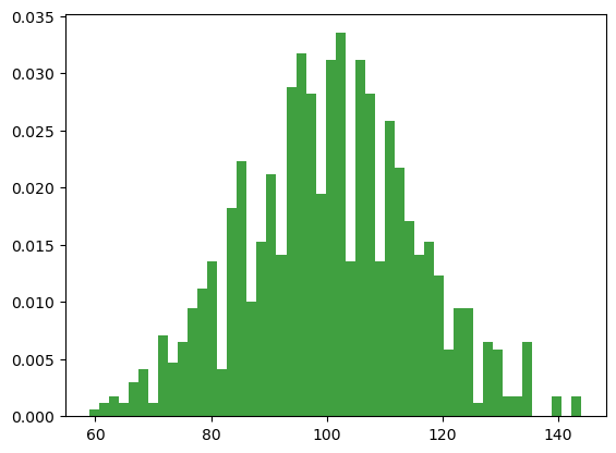
Each of these IQ scores is sampled from a normal distribution with mean 100 and standard deviation 15. So if I plot a histogram of the sample, I get roughly the right shape, but a crude approximation to the true population distribution.
In this case, the people in the sample have a mean IQ of 98.5, with sd 15.9. These sample statistics are properties of the data set, and although similar to the true population values, they are not the same.
In general, sample statistics are the things you can calculate from your data set, and the population parameters are the things you want to learn about.
The law of large numbers
Suppose that we ran a much larger experiment, this time measuring the IQ’s of 10,000 people.
We can simulate the results of this experiment using Python, using the numpy normal() function which I usually import from the numpy.random submodule using import numpy.random as npr, which generates random numbers sampled from a normal distribution.
For an experiment with a sample size of size = 10000, and a population with loc = 100 (i.e, the location of the mean) and sd = 15 (referred to as scale here), python produces our fake IQ data using these commands:
import numpy as np
import numpy.random as npr
import matplotlib.pyplot as plt
IQ = npr.normal(loc=100, scale=15, size=1000) # generate IQ scores
IQ = np.round(IQ, decimals=0)
We can compute the mean IQ using the command np.mean(IQ) and the standard deviation using the command np.std(IQ), and draw a histogram using plt.hist().
print(np.mean(IQ))
100.379
print(np.std(IQ))
14.938318479668318
n, bins, patches = plt.hist(IQ, 50, density=True, facecolor='g', alpha=0.75)

law of large numbers: a mathematical law that applies to many sample statistics
For example, when applied to the sample mean, the law of large numbers states that as the sample gets larger, the sample mean tends to get closer to the true population mean.
Or, to say it a little bit more precisely, as the sample size “approaches” infinity (written as 𝑁→∞) the sample mean approaches the population mean (𝑋→𝜇)
While descriptive statistics are nice they are usually not what we want to know when we conduct a research study.
Instead we are interested in estimation of aspects (we’ll call them parameters) of the population.
We’re using the sample mean as the best guess of the population mean
A sample statistic is a description of your data, whereas the estimate is a guess about the population (different notations)
Estimating aspects of the population
Estimating the standard deviation of the population
The sample std is a biased estimator of the population std. The sample gets closer to the population as N increases.
Simple fix to transform it into unbiased est:
2. The Bayesian view#
Also called the subjectivist view
Minority view amongst statisticians, but becoming more and more popular Defines probability of an event as the degree of belief that a rational agent assigns to the truth of that event.
Example: Suppose that I believe that there’s a 60% probability of rain tomorrow. If someone offers me a bet: if it rains tomorrow, then I win 5 dollars, but if it doesn’t rain then I lose 5 dollars
“Subjective probability” == what bets I’m willing to accept
The set of all possible events X is called a sample space.
For an event X, the probability of that event P(X) is a number that lies between 0 and 1.
The law of total probability: The probabilities of the elementary events X need to add up to 1.
Basic rules probabilities satisfy:
Probability distributions#
Examples: Binomial, Normal, t-distribution, chi-square, F distribution.
Other examples: Gamma, Poisson
Binomial distribution [X ~ Binomial (θ, N)]
N is the number of dice rolls, θ is to the the probability that a die comes up heads
The binomial distribution is the discrete probability distribution of the number of successes in a sequence of n independent experiments, each asking a yes-no question, and each with its own outcome: success (with probability p) or failure (with probability q = 1 - p).
A single success/failure experiment is also called a Bernoulli trial; for a single trial, i.e., n = 1, the binomial distribution is a Bernoulli distribution.
Normal distribution [X ~ Normal (μ, σ)]
The normal distribution, which is also referred to as “the bell curve” or a “Gaussian distribution”, is described using two parameters, the mean μ and the standard deviation σ
T-distribution
The t-distribution looks very similar to a normal distribution, but has heavier tails
This distribution is used in situations where you think that the data follow a normal distribution, but you don’t know the mean or standard deviation.
Chi-square distribution
The χ2 distribution is useful for categorical data analysis.
F-distribution
The F distribution is useful when comparing two chi square distributions to each other.
Poisson distribution
Poisson distribution is used for count data
Examples: the number of cases of cancer in a county, or the number of hits to a website during a particular hour, or the number of mass shootings in a state.
Random variables vs manipulated variables#
A random variable is a quantity that is not known exactly prior to data collection.
E.g. anxiety on any given day for a randomly selected pp
A manipulated variable is a quantity that is determined by a sampling plan or an experimental design.
E.g. Day to exam, gender, age, SES
Expectation & variance operators#
Expectation operators: definitions
The population mean, μ = E(X), is the average of all elements in the population.
It can be derived knowing only the form of the population distribution.
Let f(X) be the density function describing the likelihood of different values of X in the population.
The population mean is the average of all values of X weighted by the likelihood of each value.
If X has finite discrete values, each with probability f(X)=P(X), E(X)=Σ P(\(x_{i}\))\(x_{i}\)
If X has continuous values, we write E(X)= ∫ x f(x) dx
Expectation operators assume that f(X), f(Y) and f(X,Y) can be known, but they do not assume that these describe bell shape or normal distributions
Expectation operators: rules
E(X)=μx is the first moment, the mean
Let k represent some constant number (not random)
E(k * X) = k * E(X) = k * \(μ_{x}\)
E(X+k) = E(X)+k = \(μ_{x}\)+k
Let Y represent another random variable (perhaps related to X)
E(X+Y) = E(X)+E(Y) = \(μ_{x}\) + \(μ_{y}\)
E(X-Y) = E(X)-E(Y) = \(μ_{x}\) - \(μ_{y}\)
E( ) = E[(\(X_{1}\)+\(X_{2}\))/2] =(\(μ_{1}\) + \(μ_{2}\))/2 = μ The expected value of the average of two random variables is the average of their means.
Variance operators
Analogous to E(Y)=μ, is V(Y)=E\((Y-μ)^{2}\) = ∫ \((y - μ)^{2}\)f(y) dy
E[(X-\(μ_{x}\))\(^{2}\)] = V(X) = \(σ_{x}^{2}\)
Let k represent some constant
V(k * X) = k\(^{2}\) * V(X) = k\(^{2}\) * \(σ_{x}^{2}\)
V(X+k) = V(X) = \(σ_{x}^{2}\)
Let Y represent another random variable that is independent of X
V(X+Y) = V(X)+V(Y) = \(σ_{x}^{2}\) + \(σ_{y}^{2}\)
V(X-Y) = V(X)+V(Y) = \(σ_{x}^{2}\) + \(σ_{y}^{2}\)
Covariance & unbiased estimators#
Covariance
E[(X-\(μ_{x}\))(Y-\(μ_{y}\))] = Cov(X,Y) = σ\(_{XY}\) is the population covariance.
Covariance is the average product of deviations from means.
Covariance is zero when the variables are linearly independent.
Formally it depends on the joint bivariate density of X and Y, f(X,Y).
Cov(X,Y)= ∫ ∫(X-\(μ_{x}\))(Y-\(μ_{y}\))f(X,Y)dXdY
Unbiased estimators
Let X be the sample average of n random variables that are independently sampled from the same distribution (i.i.d) (The expected mean of each X is the same, as is the expected variance).
Because the expectation of the sample mean is equal to the parameter it is estimating, we say it is unbiased.
The expected variance of the sample mean goes down directly with increased sample size, n.
Assumed iid observations
The square root of this variance is the standard error of the mean (SE)
