Regression#
Notebook created for Regression in Psychology PSYCH–GA.2229 graduate level course at New York University by Dr. Madalina Vlasceanu
This content is Open Access (free access to information and unrestricted use of electronic resources for everyone).
Sources:
Navarro, D. (2013). Learning statistics with R: https://learningstatisticswithr.com/
Gureckis, 2018 https://teaching.gureckislab.org/fall22/labincp/intro.html
Linear regression is the standard tool for analyzing the relation between interval scale predictors (IVs) and interval scale outcomes (DVs). Formula for a straight line: y=mx+c
m is slope of the line
if you change x by 1 unit, y changes by m units
c is the y-intercept of the line
c is also the value of y when x=0
Hypothesis tests for regression models:
Does the regression model perform better than a null model?
Is a particular regression coefficient different from 0?
# import libraries

import numpy as np
import statsmodels.api as sm
import pandas as pd
import seaborn as sns
import matplotlib.pyplot as plt
import scipy.stats as stats
import statsmodels.formula.api as smf
from sklearn.linear_model import LinearRegression
from statsmodels.stats.outliers_influence import OLSInfluence
from statsmodels.formula.api import ols
from statsmodels.stats.outliers_influence import variance_inflation_factor
from patsy import dmatrices
from sklearn import linear_model
import statsmodels.stats.api as sms
from statsmodels.compat import lzip
from scipy.stats import bartlett
from statsmodels.stats import diagnostic as diag
from patsy.contrasts import Sum
# import data downloaded from https://github.com/mvlasceanu/RegressionData/blob/main/data.xlsx
# df = pd.read_excel('data.xlsx')

# Or you can read the Excel file directly from the URL
url = 'https://github.com/mvlasceanu/RegressionData/raw/main/data.xlsx'
df = pd.read_excel(url)

df
| Response ID | GENDER | AGE | PARTY | TRUST | RU1 | RU2 | RU3 | RU4 | ... | Post23 | Post24 | Post25 | Post26 | Post27 | Post28 | Post29 | Post30 | Post31 | Post32 | ||
|---|---|---|---|---|---|---|---|---|---|---|---|---|---|---|---|---|---|---|---|---|---|
| 0 | R_0cj5dsJg2wfpiuJ | 1 | 18 | 1 | 0 | 95 | 4.0 | 26 | 0 | -5 | ... | 69 | 60 | 20 | 58 | 84 | 22 | 42 | 77 | 90 | 71 |
| 1 | R_0rkhLjwWPHHjnTX | 0 | 19 | 2 | 1 | 76 | -5.0 | 16 | 3 | -1 | ... | 58 | 82 | 38 | 61 | 36 | 40 | 62 | 68 | 46 | 43 |
| 2 | R_10BMNpjhInMfUeO | 1 | 18 | 1 | 1 | 86 | -5.0 | -2 | 5 | 5 | ... | 35 | 46 | 39 | 65 | 44 | 42 | 53 | 55 | 45 | 35 |
| 3 | R_120iGR6WlLnbZnI | 0 | 22 | 1 | 0 | 95 | 23.0 | -10 | -40 | 22 | ... | 14 | 76 | 20 | 61 | 87 | 82 | 63 | 19 | 97 | 37 |
| 4 | R_12qW8cDY0bNlId2 | 0 | 19 | 3 | 0 | 76 | 18.0 | -12 | 1 | 16 | ... | 17 | 81 | 31 | 83 | 82 | 76 | 43 | 33 | 82 | 47 |
| ... | ... | ... | ... | ... | ... | ... | ... | ... | ... | ... | ... | ... | ... | ... | ... | ... | ... | ... | ... | ... | ... |
| 195 | R_xapQxguTwA3Juh3 | 1 | 18 | 1 | 0 | 76 | -13.0 | 3 | 3 | -32 | ... | 56 | 69 | 2 | 68 | 68 | 61 | 71 | 17 | 82 | 27 |
| 196 | R_XMS13V10vkvYag9 | 1 | 18 | 3 | 0 | 76 | -12.0 | 5 | -7 | -4 | ... | 44 | 44 | 26 | 40 | 34 | 37 | 35 | 65 | 44 | 35 |
| 197 | R_ykkxJ7f40bzTEaZ | 1 | 19 | 1 | 0 | 89 | -3.0 | 14 | 14 | -13 | ... | 57 | 23 | 26 | 83 | 44 | 44 | 66 | 35 | 32 | 75 |
| 198 | R_ZDXFN47SOcbCJpv | 0 | 21 | 2 | 0 | 100 | 10.0 | 15 | -3 | 5 | ... | 33 | 29 | 66 | 77 | 64 | 69 | 24 | 23 | 81 | 24 |
| 199 | R_ZpYHWVd91u6fjBT | 0 | 19 | 1 | 0 | 66 | 7.0 | 27 | 11 | 39 | ... | 56 | 40 | 26 | 37 | 35 | 9 | 24 | 37 | 33 | 67 |
200 rows × 102 columns
Ordinary least squares (OLS) Regression#
# Make a simple regression plot

# Create the figure
fig, ax = plt.subplots(1,1, figsize=(5,4))

# Plot the line
sns.regplot(x=df.AGE, y=df.TRUST, scatter_kws={"color": "#C06C84","alpha":.3}, \
                                  line_kws={"color":"#7D0552","alpha":1,"lw":4}, ax=ax)

# Label the x and y axis
ax.set_ylabel('Trust in science', labelpad=10)
ax.set(xlabel='Age')

# Include this command such that all the elements of the plot appear in the figure
plt.tight_layout()

# Save figure
# plt.savefig('figure.tif', dpi=300, format="tiff")
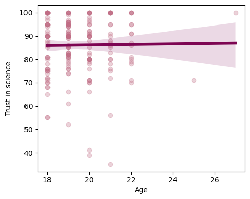
# Run a linear regression (OLS) using age to predict trust in science

md = smf.ols("TRUST ~ AGE", df)
mdf = md.fit()
print(mdf.summary())
                            OLS Regression Results
==============================================================================
Dep. Variable:                  TRUST   R-squared:                       0.000
Model:                            OLS   Adj. R-squared:                 -0.005
Method:                 Least Squares   F-statistic:                   0.03188
Date:                Sun, 04 Feb 2024   Prob (F-statistic):              0.858
Time:                        17:02:19   Log-Likelihood:                -785.74
No. Observations:                 200   AIC:                             1575.
Df Residuals:                     198   BIC:                             1582.
Df Model:                           1
Covariance Type:            nonrobust
==============================================================================
                 coef    std err          t      P>|t|      [0.025      0.975]
------------------------------------------------------------------------------
Intercept     83.9158     12.237      6.858      0.000      59.785     108.047
AGE            0.1118      0.626      0.179      0.858      -1.123       1.346
==============================================================================
Omnibus:                       49.394   Durbin-Watson:                   2.264
Prob(Omnibus):                  0.000   Jarque-Bera (JB):               90.748
Skew:                          -1.231   Prob(JB):                     1.97e-20
Kurtosis:                       5.196   Cond. No.                         274.
==============================================================================

Notes:
[1] Standard Errors assume that the covariance matrix of the errors is correctly specified.
Report regression result:
“Age was not a significant predictor of trust in science β=0.11, SE=0.62, t(198)=0.179, p=0.858.”
Other important interpretations from this OLS output:
Age explains 0% (this is the R squared value) of the variance of trust in science
the intercept (here 83.9) is the value of trust in science (y) when age (x) is 0
fig, ax = plt.subplots(1,1, figsize=(4,5))
sns.barplot(x=df.PARTY, y=df.TRUST, ax=ax)
plt.ylim(60,100)
(60.0, 100.0)
# Run a multiple linear regression (OLS) using age and gender and party affiliation to predict trust in science in the same model

md = smf.ols("TRUST ~ C(PARTY)", df)
mdf = md.fit()
print(mdf.summary())
                            OLS Regression Results
==============================================================================
Dep. Variable:                  TRUST   R-squared:                       0.077
Model:                            OLS   Adj. R-squared:                  0.067
Method:                 Least Squares   F-statistic:                     8.174
Date:                Sun, 04 Feb 2024   Prob (F-statistic):           0.000389
Time:                        17:02:19   Log-Likelihood:                -777.79
No. Observations:                 200   AIC:                             1562.
Df Residuals:                     197   BIC:                             1571.
Df Model:                           2
Covariance Type:            nonrobust
=================================================================================
                    coef    std err          t      P>|t|      [0.025      0.975]
---------------------------------------------------------------------------------
Intercept        88.5906      1.057     83.812      0.000      86.506      90.675
C(PARTY)[T.2]    -9.1144      2.806     -3.248      0.001     -14.648      -3.581
C(PARTY)[T.3]    -5.9175      1.961     -3.017      0.003      -9.785      -2.050
==============================================================================
Omnibus:                       27.642   Durbin-Watson:                   2.261
Prob(Omnibus):                  0.000   Jarque-Bera (JB):               35.982
Skew:                          -0.882   Prob(JB):                     1.54e-08
Kurtosis:                       4.097   Cond. No.                         3.60
==============================================================================

Notes:
[1] Standard Errors assume that the covariance matrix of the errors is correctly specified.
Important interpretations from this OLS output:
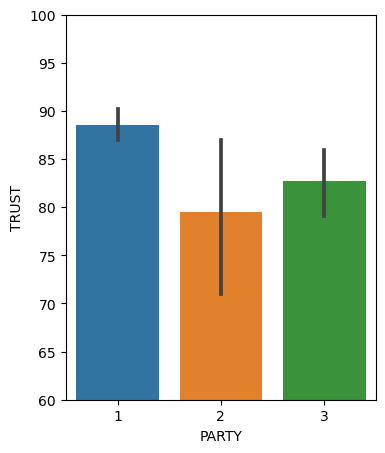
Political party explains 7% (this is the R squared value) of the variance of trust in science
the F statistic (and its associated p value) are testing the entire model against the null hypohtesis that nothing you included as predictors in this model explains any variance of the Outcome variable (DV, here trust in science)
the intercept (here 88.5) is the value of trust in science (y) when Party takes on the baseline (or first, in order) value (here the first value of party is 1, which codes for Democrats); you can also see this in the plot above;
the coefficients of the other two party categories are now the differences from the baseline one; so for Party==2 (which means Republican) the mean is 88.5 mius 9.11; then all the statistics that follow are those of an independent sample t-test, testing the difference between the baseline mean (trust in science of Democrats) and this mean (trust in science of Republicans);
the same logic applies for Party==3, which is also being compared to the baseline (here baseline is Party==1 or Democrats).
if you want to change the baseline, simply dummy code another level of this variable to be first (either numerically or alphabetically)
Ordinary least squares (OLS) Multiple Regression#
# Run a multiple linear regression (OLS) using age and gender and party affiliation to predict trust in science in the same model

md = smf.ols("TRUST ~ AGE + C(GENDER) + C(PARTY)", df)
mdf = md.fit()
print(mdf.summary())
                            OLS Regression Results
==============================================================================
Dep. Variable:                  TRUST   R-squared:                       0.081
Model:                            OLS   Adj. R-squared:                  0.063
Method:                 Least Squares   F-statistic:                     4.321
Date:                Sun, 04 Feb 2024   Prob (F-statistic):            0.00227
Time:                        17:02:19   Log-Likelihood:                -777.27
No. Observations:                 200   AIC:                             1565.
Df Residuals:                     195   BIC:                             1581.
Df Model:                           4
Covariance Type:            nonrobust
==================================================================================
                     coef    std err          t      P>|t|      [0.025      0.975]
----------------------------------------------------------------------------------
Intercept         91.1421     13.105      6.955      0.000      65.296     116.988
C(GENDER)[T.1]    -1.8577      1.902     -0.977      0.330      -5.609       1.894
C(PARTY)[T.2]     -9.3544      2.824     -3.313      0.001     -14.924      -3.785
C(PARTY)[T.3]     -6.2136      1.988     -3.126      0.002     -10.134      -2.293
AGE               -0.0642      0.644     -0.100      0.921      -1.335       1.206
==============================================================================
Omnibus:                       28.509   Durbin-Watson:                   2.260
Prob(Omnibus):                  0.000   Jarque-Bera (JB):               37.474
Skew:                          -0.901   Prob(JB):                     7.29e-09
Kurtosis:                       4.119   Cond. No.                         305.
==============================================================================

Notes:
[1] Standard Errors assume that the covariance matrix of the errors is correctly specified.
In this multiple regression above, we are testing the effects of age (as a continuous variable), gender (categorical), and party (categorical) on trust in science. We use plus sign indicating we only care about main effects, no interactions yet. Now, the intercept represents the value of trust in science (y) when all the predictors are 0 (x==0) – that is, when gender takes on the first value (here the first is 0, which means “men”), and party takes on the first value (here the first is 1 which means “Democrat”), and age is 0 - in other words, the intercept here tells you that for Democratic men, the best fit regression line between age and trust in scinece intersects the x=0 line at 91.14. This interpretation is not always meaningful.
# Run a multiple linear regression (OLS) using age and gender and party affiliation to predict trust in science in the same model

md = smf.ols("TRUST ~ AGE + C(GENDER)", df)
mdf = md.fit()
print(mdf.summary())
                            OLS Regression Results
==============================================================================
Dep. Variable:                  TRUST   R-squared:                       0.001
Model:                            OLS   Adj. R-squared:                 -0.009
Method:                 Least Squares   F-statistic:                   0.07964
Date:                Sun, 04 Feb 2024   Prob (F-statistic):              0.923
Time:                        17:02:19   Log-Likelihood:                -785.68
No. Observations:                 200   AIC:                             1577.
Df Residuals:                     197   BIC:                             1587.
Df Model:                           2
Covariance Type:            nonrobust
==================================================================================
                     coef    std err          t      P>|t|      [0.025      0.975]
----------------------------------------------------------------------------------
Intercept         85.9607     13.535      6.351      0.000      59.269     112.652
C(GENDER)[T.1]    -0.6962      1.949     -0.357      0.721      -4.541       3.148
AGE                0.0299      0.668      0.045      0.964      -1.287       1.347
==============================================================================
Omnibus:                       49.658   Durbin-Watson:                   2.267
Prob(Omnibus):                  0.000   Jarque-Bera (JB):               91.543
Skew:                          -1.236   Prob(JB):                     1.32e-20
Kurtosis:                       5.208   Cond. No.                         303.
==============================================================================

Notes:
[1] Standard Errors assume that the covariance matrix of the errors is correctly specified.
Report result:
“In a multiple linear regression model with trust in science as the DV (outcome), and age, gender, and political party affiliation as the IVs (predictors), we found no significant differences between men and women in trust in science (p=0.33), and no significant effect of age on trust in science (p=0.92); however we did find a significant difference between democrats and republicans, such that republicans trust in science significantly less than democrats (β=–9.35, SE=2.82, t(195)=–3.31, p<0.001), and a significant difference between Democrats and Independents, such that independents also trust in science significantly less than Democrats (β=–6.21, SE=1.98, t(195)=–3.12, p=0.002).”
Interaction // Moderation#
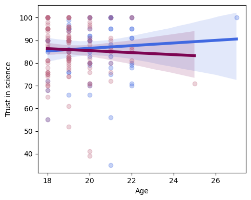
fig, ax = plt.subplots(1,1, figsize=(5,4))

#plot age predicting trust in science but only for men (gender==0)
sns.regplot(x=df.query('GENDER == 0')['AGE'], y=df.query('GENDER == 0')['TRUST'], scatter_kws={"color": "#4169E1","alpha":.3}, \
                                  line_kws={"color":"#4169E1","alpha":1,"lw":4}, ax=ax)

#plot age predicting trust in science but only for women (gender==1)
sns.regplot(x=df.query('GENDER == 1')['AGE'], y=df.query('GENDER == 1')['TRUST'], scatter_kws={"color": "#C06C84","alpha":.3}, \
                                  line_kws={"color":"#7D0552","alpha":1,"lw":4}, ax=ax)
ax.set_ylabel('Trust in science', labelpad=10)
ax.set(xlabel='Age')
plt.tight_layout()
# Run a linear regression (OLS) using age as it interacts with gender to predict trust in science

md = smf.ols("TRUST ~ AGE*C(GENDER)", df)
mdf = md.fit()
print(mdf.summary())
                            OLS Regression Results
==============================================================================
Dep. Variable:                  TRUST   R-squared:                       0.004
Model:                            OLS   Adj. R-squared:                 -0.011
Method:                 Least Squares   F-statistic:                    0.2475
Date:                Sun, 04 Feb 2024   Prob (F-statistic):              0.863
Time:                        17:02:20   Log-Likelihood:                -785.38
No. Observations:                 200   AIC:                             1579.
Df Residuals:                     196   BIC:                             1592.
Df Model:                           3
Covariance Type:            nonrobust
======================================================================================
                         coef    std err          t      P>|t|      [0.025      0.975]
--------------------------------------------------------------------------------------
Intercept             74.8330     19.893      3.762      0.000      35.600     114.066
C(GENDER)[T.1]        19.4725     26.473      0.736      0.463     -32.736      71.681
AGE                    0.5824      0.985      0.591      0.555      -1.360       2.525
AGE:C(GENDER)[T.1]    -1.0249      1.342     -0.764      0.446      -3.671       1.621
==============================================================================
Omnibus:                       50.038   Durbin-Watson:                   2.278
Prob(Omnibus):                  0.000   Jarque-Bera (JB):               92.737
Skew:                          -1.242   Prob(JB):                     7.29e-21
Kurtosis:                       5.226   Cond. No.                         842.
==============================================================================

Notes:
[1] Standard Errors assume that the covariance matrix of the errors is correctly specified.
Reporting result:
“In a multiple linear regression with age and gender as predictors and trust in science as the outcome variable, we found no main effect of gender (p=0.46), no main effect of age (p=0.55), and no gender by age interaction (p=0.44).”
Example 2#
# import data downloaded from https://github.com/mvlasceanu/RegressionData/blob/main/dataB.xlsx
# df2 = pd.read_excel('dataB.xlsx')

# Or you can read the Excel file directly from the URL
url = 'https://github.com/mvlasceanu/RegressionData/raw/main/dataB.xlsx'
df2 = pd.read_excel(url)

df2
| Bchange | Cchange | IncDec | BeliefPOST | ChoicePOST | BeliefPRE | ChoicePRE | partnum | |
|---|---|---|---|---|---|---|---|---|
| 0 | 10.75 | 2.5 | 1 | 75.50 | 16.25 | 64.75 | 13.75 | 1 |
| 1 | 35.00 | 7.5 | 1 | 100.00 | 25.00 | 65.00 | 17.50 | 2 |
| 2 | 8.75 | 0.0 | 1 | 99.75 | 25.00 | 91.00 | 25.00 | 3 |
| 3 | 40.75 | 5.0 | 1 | 87.25 | 20.00 | 46.50 | 15.00 | 4 |
| 4 | 0.00 | 0.0 | 1 | 48.25 | 25.00 | 48.25 | 25.00 | 5 |
| ... | ... | ... | ... | ... | ... | ... | ... | ... |
| 361 | -17.25 | 0.0 | 0 | 25.00 | 10.00 | 42.25 | 10.00 | 179 |
| 362 | -57.50 | -15.0 | 0 | 4.25 | 0.00 | 61.75 | 15.00 | 180 |
| 363 | -25.00 | -25.0 | 0 | 25.00 | 0.00 | 50.00 | 25.00 | 181 |
| 364 | -40.50 | -25.0 | 0 | 16.75 | 0.00 | 57.25 | 25.00 | 182 |
| 365 | 7.50 | -2.5 | 0 | 33.75 | 7.50 | 26.25 | 10.00 | 183 |
366 rows × 8 columns
# Create the figure of belief change predicting choice change
fig, ax = plt.subplots(1,1, figsize=(5,4))

# Plot the line
sns.regplot(x=df2.Bchange, y=df2.Cchange, scatter_kws={"color": "#E7CDC9"}, line_kws={"color":"#900C3F"}, ax=ax)
<Axes: xlabel='Bchange', ylabel='Cchange'>
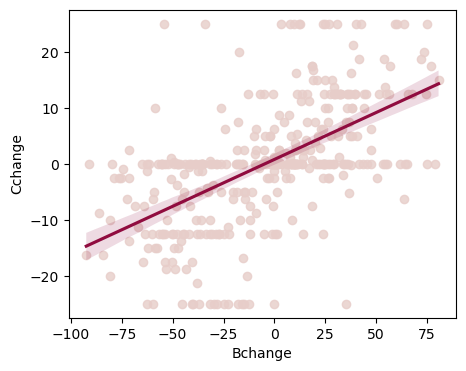
# Run a linear regression (OLS) using belief change and belief at pretest and their interaction to predict choice change

md = smf.ols("Cchange ~ Bchange", df2)
mdf = md.fit()
print(mdf.summary())
                            OLS Regression Results
==============================================================================
Dep. Variable:                Cchange   R-squared:                       0.319
Model:                            OLS   Adj. R-squared:                  0.317
Method:                 Least Squares   F-statistic:                     170.8
Date:                Sun, 04 Feb 2024   Prob (F-statistic):           2.89e-32
Time:                        17:02:20   Log-Likelihood:                -1336.1
No. Observations:                 366   AIC:                             2676.
Df Residuals:                     364   BIC:                             2684.
Df Model:                           1
Covariance Type:            nonrobust
==============================================================================
                 coef    std err          t      P>|t|      [0.025      0.975]
------------------------------------------------------------------------------
Intercept      0.7632      0.492      1.552      0.122      -0.204       1.730
Bchange        0.1674      0.013     13.068      0.000       0.142       0.193
==============================================================================
Omnibus:                        7.640   Durbin-Watson:                   1.822
Prob(Omnibus):                  0.022   Jarque-Bera (JB):               12.359
Skew:                          -0.022   Prob(JB):                      0.00207
Kurtosis:                       3.899   Cond. No.                         38.7
==============================================================================

Notes:
[1] Standard Errors assume that the covariance matrix of the errors is correctly specified.
# Run a linear regression (OLS) using belief change and belief at pretest and their interaction to predict choice change

md = smf.ols("Cchange ~ Bchange*BeliefPRE", df2)
mdf = md.fit()
print(mdf.summary())
                            OLS Regression Results
==============================================================================
Dep. Variable:                Cchange   R-squared:                       0.337
Model:                            OLS   Adj. R-squared:                  0.332
Method:                 Least Squares   F-statistic:                     61.42
Date:                Sun, 04 Feb 2024   Prob (F-statistic):           4.04e-32
Time:                        17:02:20   Log-Likelihood:                -1331.2
No. Observations:                 366   AIC:                             2670.
Df Residuals:                     362   BIC:                             2686.
Df Model:                           3
Covariance Type:            nonrobust
=====================================================================================
                        coef    std err          t      P>|t|      [0.025      0.975]
-------------------------------------------------------------------------------------
Intercept            -2.3702      1.899     -1.248      0.213      -6.104       1.363
Bchange               0.2894      0.042      6.915      0.000       0.207       0.372
BeliefPRE             0.0434      0.032      1.376      0.170      -0.019       0.105
Bchange:BeliefPRE    -0.0019      0.001     -2.892      0.004      -0.003      -0.001
==============================================================================
Omnibus:                        8.071   Durbin-Watson:                   1.887
Prob(Omnibus):                  0.018   Jarque-Bera (JB):               13.450
Skew:                           0.006   Prob(JB):                      0.00120
Kurtosis:                       3.939   Cond. No.                     9.38e+03
==============================================================================

Notes:
[1] Standard Errors assume that the covariance matrix of the errors is correctly specified.
[2] The condition number is large, 9.38e+03. This might indicate that there are
strong multicollinearity or other numerical problems.
Reporting result:
“In a multiple linear regression with belief change and belief at pretest as predictors and choice change as the outcome variable, we found a main effect of belief change (β=0.28, SE=0.04, t(362)=6.91, p<0.001), a non-significant main effect of belief at pretest (p=0.17), and a significant belief change by belief at pretest interaction (β=–0.001, SE=0.001, t(362)=–2.89, p=0.004)”
Interpretation: the slope of belief change on choice change changes as belief at pretest changes - such that the higher belief at pretest is, the less belief change predicts behavioral change.
# add a variable to the dataframe called "BeliefPRE_ms" that stores the median split of the "BeliefPRE" continuous variable

df2['BeliefPRE_ms'] = (df2.BeliefPRE > df2.BeliefPRE.median()).astype(float)
df2
| Bchange | Cchange | IncDec | BeliefPOST | ChoicePOST | BeliefPRE | ChoicePRE | partnum | BeliefPRE_ms | |
|---|---|---|---|---|---|---|---|---|---|
| 0 | 10.75 | 2.5 | 1 | 75.50 | 16.25 | 64.75 | 13.75 | 1 | 1.0 |
| 1 | 35.00 | 7.5 | 1 | 100.00 | 25.00 | 65.00 | 17.50 | 2 | 1.0 |
| 2 | 8.75 | 0.0 | 1 | 99.75 | 25.00 | 91.00 | 25.00 | 3 | 1.0 |
| 3 | 40.75 | 5.0 | 1 | 87.25 | 20.00 | 46.50 | 15.00 | 4 | 0.0 |
| 4 | 0.00 | 0.0 | 1 | 48.25 | 25.00 | 48.25 | 25.00 | 5 | 0.0 |
| ... | ... | ... | ... | ... | ... | ... | ... | ... | ... |
| 361 | -17.25 | 0.0 | 0 | 25.00 | 10.00 | 42.25 | 10.00 | 179 | 0.0 |
| 362 | -57.50 | -15.0 | 0 | 4.25 | 0.00 | 61.75 | 15.00 | 180 | 1.0 |
| 363 | -25.00 | -25.0 | 0 | 25.00 | 0.00 | 50.00 | 25.00 | 181 | 0.0 |
| 364 | -40.50 | -25.0 | 0 | 16.75 | 0.00 | 57.25 | 25.00 | 182 | 0.0 |
| 365 | 7.50 | -2.5 | 0 | 33.75 | 7.50 | 26.25 | 10.00 | 183 | 0.0 |
366 rows × 9 columns
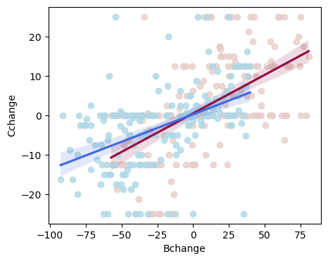
# Create the figure of belief change predicting choice change
fig, ax = plt.subplots(1,1, figsize=(5,4))

# Plot the line of belief change predicting choice change but only for the initially low pretest beliefs (BeliefPRE_ms==0)
sns.regplot(x=df2.query('BeliefPRE_ms==0')['Bchange'], y=df2.query('BeliefPRE_ms==0')['Cchange'], scatter_kws={"color": "#E7CDC9"}, line_kws={"color":"#900C3F"}, ax=ax)

# Plot the line of belief change predicting choice change but only for the initially high pretest beliefs (BeliefPRE_ms==1)
sns.regplot(x=df2.query('BeliefPRE_ms==1')['Bchange'], y=df2.query('BeliefPRE_ms==1')['Cchange'], scatter_kws={"color": "#ADD8E6"}, line_kws={"color":"#4169E1"}, ax=ax)
<Axes: xlabel='Bchange', ylabel='Cchange'>
# Now run the same linear regression as before, but now use belief change and the median split of the belief at pretest to predict choice change

md = smf.ols("Cchange ~ Bchange*C(BeliefPRE_ms)", df2)
mdf = md.fit()
print(mdf.summary())
                            OLS Regression Results
==============================================================================
Dep. Variable:                Cchange   R-squared:                       0.327
Model:                            OLS   Adj. R-squared:                  0.321
Method:                 Least Squares   F-statistic:                     58.60
Date:                Sun, 04 Feb 2024   Prob (F-statistic):           6.67e-31
Time:                        17:02:21   Log-Likelihood:                -1334.1
No. Observations:                 366   AIC:                             2676.
Df Residuals:                     362   BIC:                             2692.
Df Model:                           3
Covariance Type:            nonrobust
==================================================================================================
                                     coef    std err          t      P>|t|      [0.025      0.975]
--------------------------------------------------------------------------------------------------
Intercept                          0.4516      0.718      0.629      0.530      -0.960       1.863
C(BeliefPRE_ms)[T.1.0]            -0.2313      1.070     -0.216      0.829      -2.336       1.873
Bchange                            0.1956      0.020      9.934      0.000       0.157       0.234
Bchange:C(BeliefPRE_ms)[T.1.0]    -0.0562      0.028     -2.017      0.044      -0.111      -0.001
==============================================================================
Omnibus:                        7.212   Durbin-Watson:                   1.851
Prob(Omnibus):                  0.027   Jarque-Bera (JB):               11.350
Skew:                          -0.024   Prob(JB):                      0.00343
Kurtosis:                       3.861   Cond. No.                         110.
==============================================================================

Notes:
[1] Standard Errors assume that the covariance matrix of the errors is correctly specified.
# Now run the same linear regression as before, but now use belief change and the median split of the belief at pretest to predict choice change

md = smf.ols("Cchange ~ Bchange:C(BeliefPRE_ms)", df2)
mdf = md.fit()
print(mdf.summary())
                            OLS Regression Results
==============================================================================
Dep. Variable:                Cchange   R-squared:                       0.327
Model:                            OLS   Adj. R-squared:                  0.323
Method:                 Least Squares   F-statistic:                     88.11
Date:                Sun, 04 Feb 2024   Prob (F-statistic):           6.41e-32
Time:                        17:02:21   Log-Likelihood:                -1334.1
No. Observations:                 366   AIC:                             2674.
Df Residuals:                     363   BIC:                             2686.
Df Model:                           2
Covariance Type:            nonrobust
================================================================================================
                                   coef    std err          t      P>|t|      [0.025      0.975]
------------------------------------------------------------------------------------------------
Intercept                        0.3476      0.532      0.654      0.514      -0.698       1.393
Bchange:C(BeliefPRE_ms)[0.0]     0.1964      0.019     10.184      0.000       0.158       0.234
Bchange:C(BeliefPRE_ms)[1.0]     0.1409      0.018      7.693      0.000       0.105       0.177
==============================================================================
Omnibus:                        7.258   Durbin-Watson:                   1.853
Prob(Omnibus):                  0.027   Jarque-Bera (JB):               11.472
Skew:                          -0.020   Prob(JB):                      0.00323
Kurtosis:                       3.866   Cond. No.                         31.1
==============================================================================

Notes:
[1] Standard Errors assume that the covariance matrix of the errors is correctly specified.
# if you want to get the main effects of each of the slopes in the interaction you can run the regression for only those data:

# create new dataframes that only store the rows for which BeliefPRE_ms is 0; name that dataframe "df_pre_low"
df_pre_low = df2.loc[df2.BeliefPRE_ms==0]

# create new dataframes that only store the rows for which BeliefPRE_ms is 1; name that dataframe "df_pre_high"
df_pre_high = df2.loc[df2.BeliefPRE_ms==1]

# run the regression only on the df_pre_low dataframe (which only stores the datapoints corresponding to low initial pretest beliefs according to the median split)
md = smf.ols("Cchange ~ Bchange", df_pre_low)
mdf = md.fit()
print(mdf.summary())
                            OLS Regression Results
==============================================================================
Dep. Variable:                Cchange   R-squared:                       0.330
Model:                            OLS   Adj. R-squared:                  0.327
Method:                 Least Squares   F-statistic:                     89.72
Date:                Sun, 04 Feb 2024   Prob (F-statistic):           1.47e-17
Time:                        17:02:21   Log-Likelihood:                -679.44
No. Observations:                 184   AIC:                             1363.
Df Residuals:                     182   BIC:                             1369.
Df Model:                           1
Covariance Type:            nonrobust
==============================================================================
                 coef    std err          t      P>|t|      [0.025      0.975]
------------------------------------------------------------------------------
Intercept      0.4516      0.753      0.600      0.549      -1.033       1.936
Bchange        0.1956      0.021      9.472      0.000       0.155       0.236
==============================================================================
Omnibus:                        0.269   Durbin-Watson:                   1.776
Prob(Omnibus):                  0.874   Jarque-Bera (JB):                0.093
Skew:                           0.039   Prob(JB):                        0.955
Kurtosis:                       3.078   Cond. No.                         38.1
==============================================================================

Notes:
[1] Standard Errors assume that the covariance matrix of the errors is correctly specified.
# run the regression only on the df_pre_high dataframe (which only stores the datapoints corresponding to high initial pretest beliefs according to the median split)

md = smf.ols("Cchange ~ Bchange", df_pre_high)
mdf = md.fit()
print(mdf.summary())
                            OLS Regression Results
==============================================================================
Dep. Variable:                Cchange   R-squared:                       0.236
Model:                            OLS   Adj. R-squared:                  0.232
Method:                 Least Squares   F-statistic:                     55.62
Date:                Sun, 04 Feb 2024   Prob (F-statistic):           3.59e-12
Time:                        17:02:21   Log-Likelihood:                -653.68
No. Observations:                 182   AIC:                             1311.
Df Residuals:                     180   BIC:                             1318.
Df Model:                           1
Covariance Type:            nonrobust
==============================================================================
                 coef    std err          t      P>|t|      [0.025      0.975]
------------------------------------------------------------------------------
Intercept      0.2203      0.753      0.293      0.770      -1.265       1.705
Bchange        0.1394      0.019      7.458      0.000       0.103       0.176
==============================================================================
Omnibus:                       11.950   Durbin-Watson:                   1.905
Prob(Omnibus):                  0.003   Jarque-Bera (JB):               29.187
Skew:                          -0.109   Prob(JB):                     4.59e-07
Kurtosis:                       4.950   Cond. No.                         46.3
==============================================================================

Notes:
[1] Standard Errors assume that the covariance matrix of the errors is correctly specified.
From this plot, it looks like the red line is steeper, so belief change predicts choice change more for initially low pretest beliefs compared to initially high pretest beliefs. Let’s see if this difference in slopes is significant:
Reporting result:
“In a multiple linear regression with belief change and belief at pretest (median split) as predictors and choice change as the outcome variable, we found a main effect of belief change (β=0.19, SE=0.02, t(362)=9.93, p<0.001), a non-significant main effect of belief at pretest (p=0.82), and a significant belief change by belief at pretest interaction (β=–0.05, SE=0.02, t(362)=–2.01, p=0.044)”
Interpretation: Belief change predicts choice change less for high pretest beliefs than for low pretest beliefs. Conversly, belief change predicts choice change more for low pretest beliefs than for high pretest beliefs, same conclusion we drew from the plot.
Regression assumptions#
Normality. Residuals are normally distributed. It’s ok if the IV and DV are non-normal, as long as the residuals ε are normal.
Linearity. The relationship between the IV and DV is linear.
Homogeneity of variance. Each residual is generated from a normal distribution with mean 0 and the same standard deviation σ.
Uncorrelated predictors. If you include highly correlated IVs in the model it will cause collinearity problems.
Residuals are independent of each other (there’s nothing funny going on in the residuals, like a dependency).
No bad outliers. Ensure the model is not too strongly driven by one or two weird datapoints.
# Run a linear regression (OLS) using belief change to predict choice change

md = smf.ols("Cchange ~ Bchange", df2)
mdf = md.fit()
print(mdf.summary())
                            OLS Regression Results
==============================================================================
Dep. Variable:                Cchange   R-squared:                       0.319
Model:                            OLS   Adj. R-squared:                  0.317
Method:                 Least Squares   F-statistic:                     170.8
Date:                Sun, 04 Feb 2024   Prob (F-statistic):           2.89e-32
Time:                        17:02:21   Log-Likelihood:                -1336.1
No. Observations:                 366   AIC:                             2676.
Df Residuals:                     364   BIC:                             2684.
Df Model:                           1
Covariance Type:            nonrobust
==============================================================================
                 coef    std err          t      P>|t|      [0.025      0.975]
------------------------------------------------------------------------------
Intercept      0.7632      0.492      1.552      0.122      -0.204       1.730
Bchange        0.1674      0.013     13.068      0.000       0.142       0.193
==============================================================================
Omnibus:                        7.640   Durbin-Watson:                   1.822
Prob(Omnibus):                  0.022   Jarque-Bera (JB):               12.359
Skew:                          -0.022   Prob(JB):                      0.00207
Kurtosis:                       3.899   Cond. No.                         38.7
==============================================================================

Notes:
[1] Standard Errors assume that the covariance matrix of the errors is correctly specified.
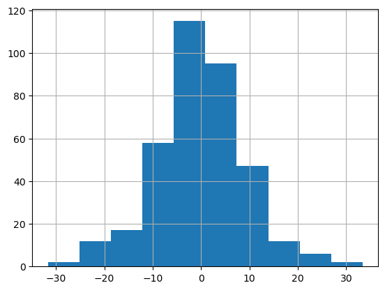
1. Normality of residuals#
# plot a histogram of the residuals, does it look normal?

mdf.resid.hist()
<Axes: >
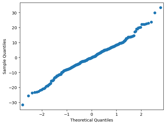
# make QQ plot to visually check if the model residuals are normally distributed
# if normally distributed, the output should be a straight diagonal line

sm.qqplot(mdf.resid)

# quantitatively test whether a variable is normally distributed using the Shapiro test
# if this test is significant, then the variable is not normally distributed

shapiro_test = stats.shapiro(mdf.resid)
shapiro_test
ShapiroResult(statistic=0.9885302186012268, pvalue=0.00559960724785924)
However, given the central limit theorem (CLT), at large sample sizes the normality assumption can be relaxed. In general, larger N is required when the errors depart more from normality (Pek, Wong, & Wong, 2018).
If however, you still want to account for this assumption, you can run a robust regression that accounts for outliers.
# Run a robust linear model

rlm_model = sm.RLM(df2.Cchange, df2.Bchange, M=sm.robust.norms.HuberT())
rlm_results = rlm_model.fit()
rlm_results.summary()
| Dep. Variable: | Cchange | No. Observations: | 366 |
|---|---|---|---|
| Model: | RLM | Df Residuals: | 365 |
| Method: | IRLS | Df Model: | 0 |
| Norm: | HuberT | ||
| Scale Est.: | mad | ||
| Cov Type: | H1 | ||
| Date: | Sun, 04 Feb 2024 | ||
| Time: | 17:02:21 | ||
| No. Iterations: | 14 |
| coef | std err | z | P>|z| | [0.025 | 0.975] | |
|---|---|---|---|---|---|---|
| Bchange | 0.1601 | 0.012 | 13.668 | 0.000 | 0.137 | 0.183 |
If the model instance has been used for another fit with different fit parameters, then the fit options might not be the correct ones anymore .
2. Linearity of relationship#
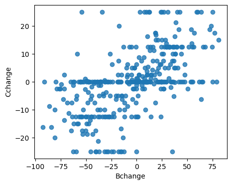
# check the correlation between the IV and DV.
# if high correlation, then relationship is likely linear

stats.pearsonr(df2.Cchange, df2.Bchange)
PearsonRResult(statistic=0.5650943589337774, pvalue=2.8890137778694925e-32)
# also visually inspect the relationship

fig, ax = plt.subplots(1,1, figsize=(5,4))
sns.regplot(x=df2.Bchange, y=df2.Cchange, fit_reg=False, ax=ax)
<Axes: xlabel='Bchange', ylabel='Cchange'>
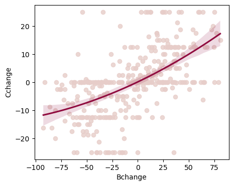
# if you suspect a quadratic relationship rather than a linear one, you can add a quadratic term to the regression
# the quadratic model is better than the linear if the AIC is lower

md = smf.ols("Cchange ~ Bchange + np.power(Bchange, 2)", df2)
mdf = md.fit()
print(mdf.summary())
                            OLS Regression Results
==============================================================================
Dep. Variable:                Cchange   R-squared:                       0.324
Model:                            OLS   Adj. R-squared:                  0.321
Method:                 Least Squares   F-statistic:                     87.13
Date:                Sun, 04 Feb 2024   Prob (F-statistic):           1.24e-31
Time:                        17:02:21   Log-Likelihood:                -1334.7
No. Observations:                 366   AIC:                             2675.
Df Residuals:                     363   BIC:                             2687.
Df Model:                           2
Covariance Type:            nonrobust
========================================================================================
                           coef    std err          t      P>|t|      [0.025      0.975]
----------------------------------------------------------------------------------------
Intercept                0.0660      0.649      0.102      0.919      -1.210       1.342
Bchange                  0.1730      0.013     13.075      0.000       0.147       0.199
np.power(Bchange, 2)     0.0005      0.000      1.643      0.101   -9.67e-05       0.001
==============================================================================
Omnibus:                        7.978   Durbin-Watson:                   1.847
Prob(Omnibus):                  0.019   Jarque-Bera (JB):               13.196
Skew:                          -0.017   Prob(JB):                      0.00136
Kurtosis:                       3.930   Cond. No.                     2.99e+03
==============================================================================

Notes:
[1] Standard Errors assume that the covariance matrix of the errors is correctly specified.
[2] The condition number is large, 2.99e+03. This might indicate that there are
strong multicollinearity or other numerical problems.
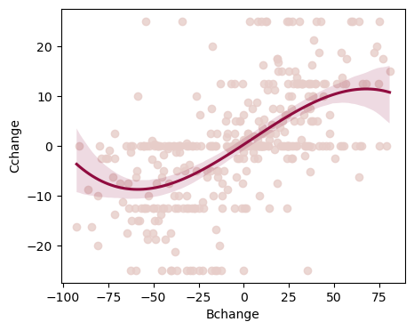
# how to plot a polinomial regression if you suspect a nonlinear relationship:
# if you think the relationship is quadratic, then include "order=2" in the the same regplot you ran for the linear plot

fig, ax = plt.subplots(1,1, figsize=(5,4))
sns.regplot(x=df2.Bchange, y=df2.Cchange, scatter_kws={"color": "#E7CDC9"}, line_kws={"color":"#900C3F"}, order=2, ax=ax)
<Axes: xlabel='Bchange', ylabel='Cchange'>
# if you think the relationship is cubic, then include "order=3" in the the same regplot you ran for the linear plot

fig, ax = plt.subplots(1,1, figsize=(5,4))
sns.regplot(x=df2.Bchange, y=df2.Cchange, scatter_kws={"color": "#E7CDC9"}, line_kws={"color":"#900C3F"}, order=3, ax=ax)
<Axes: xlabel='Bchange', ylabel='Cchange'>
3. Homogeneity of variance (Homoscedasticity)#
Each residual is generated from a normal distribution with mean 0 and the same standard deviation σ.
# check if the mean of the residuals is 0
mdf.resid.mean()
-4.08465004382309e-14
# Bartlett’s test tests the null hypothesis that all input samples are from populations with equal variances.
# if p value is less than 0.05 (significant Bartlett’s test), then the homogeneity of variance assumption is violated

test = bartlett(mdf.predict(df2.Bchange), mdf.resid)
print(test)
BartlettResult(statistic=48.00931580909055, pvalue=4.241988854393965e-12)
# because the homogeneity of variance assumption is violated, run a weighted least squares regression (WLS) instead of OLS

md = smf.wls("Cchange ~ Bchange", df2)
mdf = md.fit()
print(mdf.summary())
                            WLS Regression Results
==============================================================================
Dep. Variable:                Cchange   R-squared:                       0.319
Model:                            WLS   Adj. R-squared:                  0.317
Method:                 Least Squares   F-statistic:                     170.8
Date:                Sun, 04 Feb 2024   Prob (F-statistic):           2.89e-32
Time:                        17:02:23   Log-Likelihood:                -1336.1
No. Observations:                 366   AIC:                             2676.
Df Residuals:                     364   BIC:                             2684.
Df Model:                           1
Covariance Type:            nonrobust
==============================================================================
                 coef    std err          t      P>|t|      [0.025      0.975]
------------------------------------------------------------------------------
Intercept      0.7632      0.492      1.552      0.122      -0.204       1.730
Bchange        0.1674      0.013     13.068      0.000       0.142       0.193
==============================================================================
Omnibus:                        7.640   Durbin-Watson:                   1.822
Prob(Omnibus):                  0.022   Jarque-Bera (JB):               12.359
Skew:                          -0.022   Prob(JB):                      0.00207
Kurtosis:                       3.899   Cond. No.                         38.7
==============================================================================

Notes:
[1] Standard Errors assume that the covariance matrix of the errors is correctly specified.
# if homogeneity of variance assumption is violated and the predictors are correlated (next assumption), run Generalised Least Squares (GLS) instead:

md = smf.gls("Cchange ~ Bchange", df2)
mdf = md.fit()
print(mdf.summary())
                            GLS Regression Results
==============================================================================
Dep. Variable:                Cchange   R-squared:                       0.319
Model:                            GLS   Adj. R-squared:                  0.317
Method:                 Least Squares   F-statistic:                     170.8
Date:                Sun, 04 Feb 2024   Prob (F-statistic):           2.89e-32
Time:                        17:02:23   Log-Likelihood:                -1336.1
No. Observations:                 366   AIC:                             2676.
Df Residuals:                     364   BIC:                             2684.
Df Model:                           1
Covariance Type:            nonrobust
==============================================================================
                 coef    std err          t      P>|t|      [0.025      0.975]
------------------------------------------------------------------------------
Intercept      0.7632      0.492      1.552      0.122      -0.204       1.730
Bchange        0.1674      0.013     13.068      0.000       0.142       0.193
==============================================================================
Omnibus:                        7.640   Durbin-Watson:                   1.822
Prob(Omnibus):                  0.022   Jarque-Bera (JB):               12.359
Skew:                          -0.022   Prob(JB):                      0.00207
Kurtosis:                       3.899   Cond. No.                         38.7
==============================================================================

Notes:
[1] Standard Errors assume that the covariance matrix of the errors is correctly specified.
5. Residuals are independent#
# check for autocorrelation
# to ensure the absence of autocorrelation we use Ljungbox test.
# Null Hypothesis: Autocorrelation is absent.
# Alternative Hypothesis: Autocorrelation is present.

min(diag.acorr_ljungbox(mdf.resid , lags = 40, return_df=False))
'lb_pvalue'
# because it seems from the test above that my residuals are not independent, one solution is to run a GLSAR instead
# GLSAR is a feasible generalized least squares with autocorrelated AR(p) errors
# this is how you run it:

Y = df2.Cchange
X = df2.Bchange
X = sm.add_constant(X)
model2 = sm.GLSAR(Y, X, rho=2)
results = model2.iterative_fit(maxiter=6)
model2.rho
print("Coefficients:\n", results.params)
print("Coefficient t-values\n", results.tvalues)
print("Coefficient t-tests?\n", results.t_test([[1, 0], [0, 1]]))
Coefficients:
 const      0.717936
Bchange    0.159007
dtype: float64
Coefficient t-values
 const       1.283222
Bchange    11.624478
dtype: float64
Coefficient t-tests?
                              Test for Constraints
==============================================================================
                 coef    std err          t      P>|t|      [0.025      0.975]
------------------------------------------------------------------------------
c0             0.7179      0.559      1.283      0.200      -0.382       1.818
c1             0.1590      0.014     11.624      0.000       0.132       0.186
==============================================================================
6. No bad outliers#
# Cook’s distance

# create instance of influence
# influence = mdf.get_influence()

# get Cook's distance for each observation
# cooks_distances, pval = influence.cooks_distance

# print Cook's distances (an array of values for Cook’s distance for each observation and a corresponding array of p-values)
# sigificant p-values means the outlier is bad
# print(cooks_distances)
# print(pval)
# visualize the outliers to spot the bad ones
# consider removing the bad outliers to improve the model fit (but this decision depends on your research question)

# plt.s# catter(df2.Bchange, pval)
# plt.s# how()
# if you want to remove the sigificantly bad outliers (as determined by the pvalues of Cook's distnace) from the dataframe:
# uset the loc function to only keep the observations that are not significant outliers

# df2 = df2.loc[pval>=0.05]
# if your data has bad outliers but you don't want to remove them, run a robust linear model (RLM):

rlm_model = sm.RLM(df2.Cchange, df2.Bchange, M=sm.robust.norms.HuberT())
rlm_results = rlm_model.fit()
rlm_results.summary()
| Dep. Variable: | Cchange | No. Observations: | 366 |
|---|---|---|---|
| Model: | RLM | Df Residuals: | 365 |
| Method: | IRLS | Df Model: | 0 |
| Norm: | HuberT | ||
| Scale Est.: | mad | ||
| Cov Type: | H1 | ||
| Date: | Sun, 04 Feb 2024 | ||
| Time: | 17:02:24 | ||
| No. Iterations: | 14 |
| coef | std err | z | P>|z| | [0.025 | 0.975] | |
|---|---|---|---|---|---|---|
| Bchange | 0.1601 | 0.012 | 13.668 | 0.000 | 0.137 | 0.183 |
If the model instance has been used for another fit with different fit parameters, then the fit options might not be the correct ones anymore .
Regression power analysis#
Compute power: WebPower: https://webpower.psychstat.org/wiki/models/index
