T-Test#
Notebook created for Regression in Psychology PSYCH–GA.2229 graduate level course at New York University by Dr. Madalina Vlasceanu
This content is Open Access (free access to information and unrestricted use of electronic resources for everyone).
Sources:
Navarro, D. (2013). Learning statistics with R: https://learningstatisticswithr.com/
Gureckis, 2018 https://teaching.gureckislab.org/fall22/labincp/intro.html
T-Test#
The T-test (or Student’s t-test) tests if there is a difference between two continuous variables’ means.
Therefore, the predictor (IV) is categorical, but the outcome (DV) is continuous.
There are 3 Types of t-tests:
One sample t-test - compares a mean to a number
Independent sample t-test - compares two means from different groups
Paired sample t-test - compares two means from same group (pre-post)
# import libraries

import numpy as np
import statsmodels.api as sm
import pylab as py
import pandas as pd
import seaborn as sns
import matplotlib.pyplot as plt
import scipy.stats as stats
from scipy.stats import wilcoxon
# import data downloaded from https://github.com/mvlasceanu/RegressionData/blob/main/data.xlsx
#df = pd.read_excel('data.xlsx')

# Or you can read the Excel file directly from the URL
url = 'https://github.com/mvlasceanu/RegressionData/raw/main/data.xlsx'
df = pd.read_excel(url)

df.head(2)
| Response ID | GENDER | AGE | PARTY | TRUST | RU1 | RU2 | RU3 | RU4 | ... | Post23 | Post24 | Post25 | Post26 | Post27 | Post28 | Post29 | Post30 | Post31 | Post32 | ||
|---|---|---|---|---|---|---|---|---|---|---|---|---|---|---|---|---|---|---|---|---|---|
| 0 | R_0cj5dsJg2wfpiuJ | 1 | 18 | 1 | 0 | 95 | 4.0 | 26 | 0 | -5 | ... | 69 | 60 | 20 | 58 | 84 | 22 | 42 | 77 | 90 | 71 |
| 1 | R_0rkhLjwWPHHjnTX | 0 | 19 | 2 | 1 | 76 | -5.0 | 16 | 3 | -1 | ... | 58 | 82 | 38 | 61 | 36 | 40 | 62 | 68 | 46 | 43 |
2 rows × 102 columns
# create a new variable "trustD" that selects the trust in science "TRUST" of all Democrats ('PARTY==1')
trustD = df.query('PARTY==1')['TRUST']

# create a new variable "trustr" that selects the trust in science "TRUST" of all Republicans ('PARTY==2')
trustR = df.query('PARTY==2')['TRUST']
1 Sample t-test#
The one sample t-test compares a mean to a number.
Example: Do Democrats trust in science (above chance, if chance is 75)?#
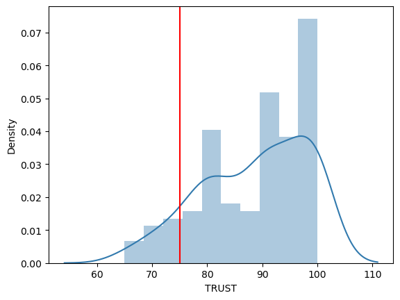
In other words, is the mean of Democrats’ trust in science higher than 75?
# plot the distribution of trustD

# create a figure with one by one panels
fig, ax = plt.subplots(1,1)

# plot the histogram of trustD using distplot in the library seaborn
sns.distplot(trustD, hist=True, norm_hist=True, kde=True, bins=10, color = '#327AAE', ax=ax)

# you can draw a line through the x=75 to see what you are comparing the distribution of trustD to
plt.axvline(x = 75, color = 'r', label = 'axvline - full height')

#save the figure
plt.savefig('trustD.png', dpi=300, format="png")
C:\Users\kay\AppData\Local\Temp\ipykernel_24564\914974243.py:7: UserWarning:

`distplot` is a deprecated function and will be removed in seaborn v0.14.0.

Please adapt your code to use either `displot` (a figure-level function with
similar flexibility) or `histplot` (an axes-level function for histograms).

For a guide to updating your code to use the new functions, please see
https://gist.github.com/mwaskom/de44147ed2974457ad6372750bbe5751

  sns.distplot(trustD, hist=True, norm_hist=True, kde=True, bins=10, color = '#327AAE', ax=ax)
C:\ALL\AppData\anaconda3\envs\mada_book\Lib\site-packages\seaborn\_oldcore.py:1119: FutureWarning: use_inf_as_na option is deprecated and will be removed in a future version. Convert inf values to NaN before operating instead.
  with pd.option_context('mode.use_inf_as_na', True):
# check the mean of Democrats' trust in science (trustD)

trustD.mean()
88.59055118110236
# check the standard deviation (estimate of population parameter) of the variable trustD

trustD.std()
9.591956228891103
# check how many datapoints are in the variable trustD

len(trustD)
127
# compute the t statistic for a one sample ttest checking if trustD is different from 75

(88.59-75)/(9.59/np.sqrt(127))
15.969918876919223
# run the one sample ttest of whether trustD is significantly different from 75 (output is t statistic and p value)

stats.ttest_1samp(trustD, popmean=75)
TtestResult(statistic=15.967309469564503, pvalue=4.621060382873896e-32, df=126)
Assumptions of one sample t-test:
Population is normally distributed
Observations in sample are independent
# in the histogram above, it doesn't look like trustD is normally distributed
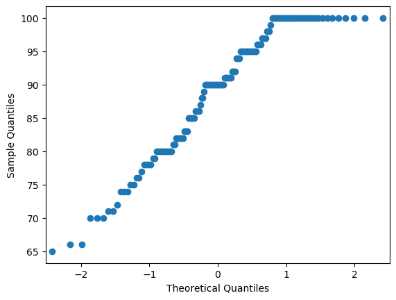
# to formally test for normality, draw a qq plot:
# if normally distributed, the output should be a straight diagonal line

sm.qqplot(trustD)
py.show()
# quantitatively test whether a variable is normally distributed using the Shapiro test
# if this test is significant, then the variable is not normally distributed

shapiro_test = stats.shapiro(trustD)
shapiro_test
ShapiroResult(statistic=0.9229094386100769, pvalue=2.0021473119413713e-06)
It looks like Democrats’ trust in science is not normally distributed in this dataset, given the non-linear looking qqplot and the sigificant Shapiro test. What now?
# for nonnormal data, instead of the one sample ttest we can run a Wilcoxon test
# Wilcoxon test is a non-parametric version of the one sample T-test
# the output is the statistic and the p value
# by default compares trustD to 0

res = wilcoxon(trustD)
res.statistic, res.pvalue
(0.0, 1.1993576441771922e-22)
# if you want to compare trustD to another number, like 75, subtract it in the test:
# compares trustD to 0

res = wilcoxon(trustD - 75)
res.statistic, res.pvalue
(229.0, 5.547779859138368e-20)
wilcoxon(trustD - 75)
WilcoxonResult(statistic=229.0, pvalue=5.547779859138368e-20)
2 Sample t-test or Independent sample t-test or Between subjects t-test#
The Independent sample t-test compares two means from different groups.
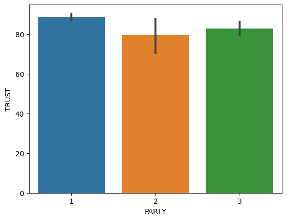
Example: Are Democrats different from Republicans in how much they trust in science?#
# make a figure that plots trust in science "TRUST" as a function of party affiliation "PARTY"

sns.barplot(x="PARTY", y="TRUST", data=df)
<Axes: xlabel='PARTY', ylabel='TRUST'>
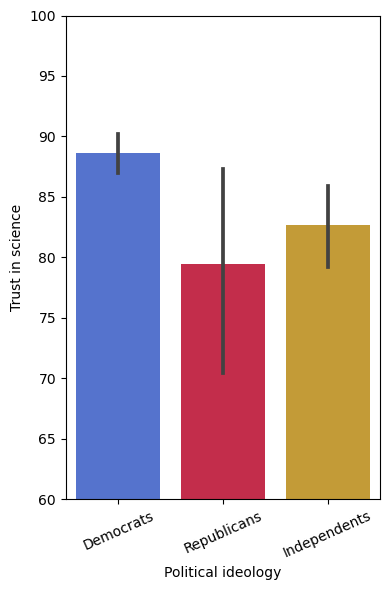
# let's make the same figure as above but customize it:

# Choose bar colors: https://sites.google.com/view/paztronomer/blog/basic/python-colors
colors = ["royalblue", "crimson", "goldenrod"]

# Create the figure specifying number of subplots and size (in inches)
fig, ax = plt.subplots(1,1, figsize=(4,6))

# Plot the bars
sns.barplot(x="PARTY", y="TRUST", data=df, palette=colors, ax=ax)

# Label the x and y axis
ax.set_ylabel('Trust in science')
ax.set_xlabel('Political ideology')
ax.set_xticklabels(['Democrats', 'Republicans', 'Independents'], rotation=24)

# Set the y limits
ax.set_ylim(60,100)

# Include this command such that all the elements of the plot appear in the figure
plt.tight_layout()
# Let's say you want to compare Democrats with Republicans on the trust in science variable
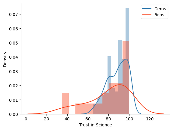
# Let's first look at the distributions of these variables

# make a figure
fig, ax = plt.subplots(1,1)

# plot Democrats' trust histogram
sns.distplot(df.query('PARTY==1')['TRUST'], hist=True, norm_hist=True, kde=True, bins=10, color = '#327AAE', ax=ax)

# plot Republicans' trust histogram in the same graph
sns.distplot(df.query('PARTY==2')['TRUST'], hist=True, norm_hist=True, kde=True, bins=10, color = '#F93F17', ax=ax)

# label the x axis
ax.set_xlabel('Trust in Science')

# include a legend
plt.legend(['Dems','Reps'])

# save the figure
plt.savefig('trust.png', dpi=300, format="png")
C:\Users\kay\AppData\Local\Temp\ipykernel_24564\3661408836.py:8: UserWarning:

`distplot` is a deprecated function and will be removed in seaborn v0.14.0.

Please adapt your code to use either `displot` (a figure-level function with
similar flexibility) or `histplot` (an axes-level function for histograms).

For a guide to updating your code to use the new functions, please see
https://gist.github.com/mwaskom/de44147ed2974457ad6372750bbe5751

  sns.distplot(df.query('PARTY==1')['TRUST'], hist=True, norm_hist=True, kde=True, bins=10, color = '#327AAE', ax=ax)
C:\ALL\AppData\anaconda3\envs\mada_book\Lib\site-packages\seaborn\_oldcore.py:1119: FutureWarning: use_inf_as_na option is deprecated and will be removed in a future version. Convert inf values to NaN before operating instead.
  with pd.option_context('mode.use_inf_as_na', True):
C:\Users\kay\AppData\Local\Temp\ipykernel_24564\3661408836.py:11: UserWarning:

`distplot` is a deprecated function and will be removed in seaborn v0.14.0.

Please adapt your code to use either `displot` (a figure-level function with
similar flexibility) or `histplot` (an axes-level function for histograms).

For a guide to updating your code to use the new functions, please see
https://gist.github.com/mwaskom/de44147ed2974457ad6372750bbe5751

  sns.distplot(df.query('PARTY==2')['TRUST'], hist=True, norm_hist=True, kde=True, bins=10, color = '#F93F17', ax=ax)
C:\ALL\AppData\anaconda3\envs\mada_book\Lib\site-packages\seaborn\_oldcore.py:1119: FutureWarning: use_inf_as_na option is deprecated and will be removed in a future version. Convert inf values to NaN before operating instead.
  with pd.option_context('mode.use_inf_as_na', True):
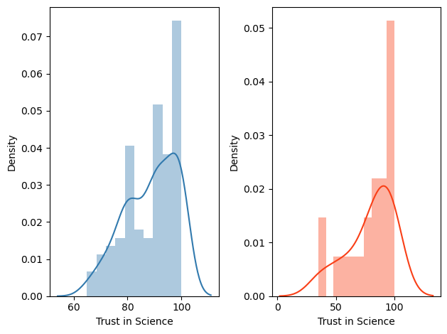
# if you want to plot the 2 distribution in separate panels

# make the figure with 2 subplots: one row and 2 columns
fig, ax = plt.subplots(1,2)

# plot Democrats' histogram in the first panel by specifying ax=ax[0]
sns.distplot(df.query('PARTY==1')['TRUST'], hist=True, norm_hist=True, kde=True, bins=10, color = '#327AAE', ax=ax[0])

# plot Republicans' histogram in the second panel by specifying ax=ax[1]
sns.distplot(df.query('PARTY==2')['TRUST'], hist=True, norm_hist=True, kde=True, bins=10, color = '#F93F17', ax=ax[1])

# label the x axis of the first and second panels
ax[0].set_xlabel('Trust in Science')
ax[1].set_xlabel('Trust in Science')

# make sure the two panels don't overlap
plt.tight_layout()

# save the figure
plt.savefig('trust.png', dpi=300, format="png")
C:\Users\kay\AppData\Local\Temp\ipykernel_24564\2675075539.py:7: UserWarning:

`distplot` is a deprecated function and will be removed in seaborn v0.14.0.

Please adapt your code to use either `displot` (a figure-level function with
similar flexibility) or `histplot` (an axes-level function for histograms).

For a guide to updating your code to use the new functions, please see
https://gist.github.com/mwaskom/de44147ed2974457ad6372750bbe5751

  sns.distplot(df.query('PARTY==1')['TRUST'], hist=True, norm_hist=True, kde=True, bins=10, color = '#327AAE', ax=ax[0])
C:\ALL\AppData\anaconda3\envs\mada_book\Lib\site-packages\seaborn\_oldcore.py:1119: FutureWarning: use_inf_as_na option is deprecated and will be removed in a future version. Convert inf values to NaN before operating instead.
  with pd.option_context('mode.use_inf_as_na', True):
C:\Users\kay\AppData\Local\Temp\ipykernel_24564\2675075539.py:10: UserWarning:

`distplot` is a deprecated function and will be removed in seaborn v0.14.0.

Please adapt your code to use either `displot` (a figure-level function with
similar flexibility) or `histplot` (an axes-level function for histograms).

For a guide to updating your code to use the new functions, please see
https://gist.github.com/mwaskom/de44147ed2974457ad6372750bbe5751

  sns.distplot(df.query('PARTY==2')['TRUST'], hist=True, norm_hist=True, kde=True, bins=10, color = '#F93F17', ax=ax[1])
C:\ALL\AppData\anaconda3\envs\mada_book\Lib\site-packages\seaborn\_oldcore.py:1119: FutureWarning: use_inf_as_na option is deprecated and will be removed in a future version. Convert inf values to NaN before operating instead.
  with pd.option_context('mode.use_inf_as_na', True):
# run an independent sample ttest (between subjects ttest) testing for differences in trust in science between Republicans and Democrats
# the output is the t statistic and the p value

stats.ttest_ind(trustD, trustR)
TtestResult(statistic=3.327609101320773, pvalue=0.0011085288899397455, df=146.0)
# Let's create a function ttest_ind that reports the Cohen D effect size, degrees of freedom, confidence intervals:

def ttest_ind(x1, x2, equivar=False, alpha=0.05, printres=False):
    n1 = len(x1)
    M1 = np.mean(x1)
    s1 = np.std(x1, ddof=1)
    n2 = len(x2)
    M2 = np.mean(x2)
    s2 = np.std(x2, ddof=1)

    # t-test
    [t, p] = stats.ttest_ind(x1, x2, equal_var=equivar)
    # cohen's d
    dof = n1 + n2 - 2
    sp = np.sqrt(((n1-1)*s1**2 + (n2-1)*s2**2) / dof)
    d = np.abs(M1 - M2) / sp
    # degrees of freedom
    df = (s1**2/n1 + s2**2/n2)**2 / ((s1**2/n1)**2/(n1-1) + (s2**2/n2)**2/(n2-1))
    # confidence intervals (M1 - M2) ± ts(M1 - M2)
    se = np.sqrt(sp**2/n1 + sp**2/n2)
    CI = (M1 - M2) + np.array([-1,1])*stats.t.ppf(1-alpha/2, df, loc=0, scale=1)*se

    res = (t, df, p, d, CI[0], CI[1])
    if printres:
        print("t = %.5f, df = %.5f, p = %.5f, d = %.5f, CI = (%.5f, %.5f)" % res)
    else:
        return res
# Run an independent sample t-test using this newly created function
res = ttest_ind(trustD, trustR)
print("t = %.5f, df = %.5f, p = %.5f, d = %.5f, CI = (%.5f, %.5f)\n" % res)
t = 2.03205, df = 21.51737, p = 0.05468, d = 0.78388, CI = (3.42660, 14.80212)
Assumptions of indepednent samples t-test:
Populations are normally distributed
Observations in samples are independent
The standard deviations are the same in both populations (homoscedasticity) - if this assumption is violated you should make sure to run the independent samples t-test Welch test. However, in Python this is the default anyway.
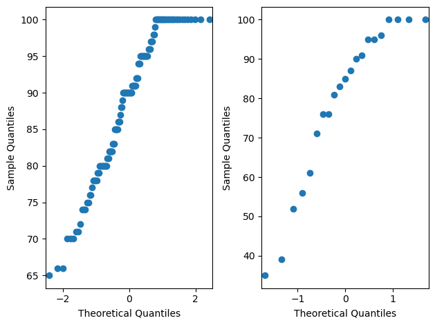
Checking for assumption of normality#
# make QQ plot to visually check if a variable is normally distributed
# if normally distributed, the output should be a straight diagonal line

fig, ax = plt.subplots(1,2)

sm.qqplot(trustD, ax=ax[0])
sm.qqplot(trustR, ax=ax[1])

plt.tight_layout()

py.show()
# quantitatively test whether a variable is normally distributed using the Shapiro test
# if this test is significant, then the variable is not normally distributed

shapiro_test = stats.shapiro(trustD)
shapiro_test
ShapiroResult(statistic=0.9229094386100769, pvalue=2.0021473119413713e-06)
# quantitatively test whether a variable is normally distributed using the Shapiro test
# if this test is significant, then the variable is not normally distributed

shapiro_test = stats.shapiro(trustR)
shapiro_test
ShapiroResult(statistic=0.8777187466621399, pvalue=0.013254587538540363)
# since trust in science is not normally distributed (as assumed by the independent sample t-test) we have to run a non parametric test instead
# one option is the Mann–Whitney U test

stats.mannwhitneyu(x=trustD, y=trustR)
MannwhitneyuResult(statistic=1612.0, pvalue=0.12441433916658333)
Paired sample t-test (Within subject t-test)#
Used for repeated measures designs (pre-post, before-after).
It’s constructed as a one-sample t-test, but applied to the difference between two variables.
Example: compare pretest beliefs to posttest beliefs, to see if the manipulation (evidence) changed participants’ beliefs
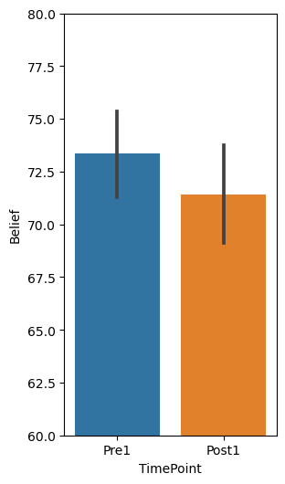
let’s first plot the variables we are comparing
df
| Response ID | GENDER | AGE | PARTY | TRUST | RU1 | RU2 | RU3 | RU4 | ... | Post23 | Post24 | Post25 | Post26 | Post27 | Post28 | Post29 | Post30 | Post31 | Post32 | ||
|---|---|---|---|---|---|---|---|---|---|---|---|---|---|---|---|---|---|---|---|---|---|
| 0 | R_0cj5dsJg2wfpiuJ | 1 | 18 | 1 | 0 | 95 | 4.0 | 26 | 0 | -5 | ... | 69 | 60 | 20 | 58 | 84 | 22 | 42 | 77 | 90 | 71 |
| 1 | R_0rkhLjwWPHHjnTX | 0 | 19 | 2 | 1 | 76 | -5.0 | 16 | 3 | -1 | ... | 58 | 82 | 38 | 61 | 36 | 40 | 62 | 68 | 46 | 43 |
| 2 | R_10BMNpjhInMfUeO | 1 | 18 | 1 | 1 | 86 | -5.0 | -2 | 5 | 5 | ... | 35 | 46 | 39 | 65 | 44 | 42 | 53 | 55 | 45 | 35 |
| 3 | R_120iGR6WlLnbZnI | 0 | 22 | 1 | 0 | 95 | 23.0 | -10 | -40 | 22 | ... | 14 | 76 | 20 | 61 | 87 | 82 | 63 | 19 | 97 | 37 |
| 4 | R_12qW8cDY0bNlId2 | 0 | 19 | 3 | 0 | 76 | 18.0 | -12 | 1 | 16 | ... | 17 | 81 | 31 | 83 | 82 | 76 | 43 | 33 | 82 | 47 |
| ... | ... | ... | ... | ... | ... | ... | ... | ... | ... | ... | ... | ... | ... | ... | ... | ... | ... | ... | ... | ... | ... |
| 195 | R_xapQxguTwA3Juh3 | 1 | 18 | 1 | 0 | 76 | -13.0 | 3 | 3 | -32 | ... | 56 | 69 | 2 | 68 | 68 | 61 | 71 | 17 | 82 | 27 |
| 196 | R_XMS13V10vkvYag9 | 1 | 18 | 3 | 0 | 76 | -12.0 | 5 | -7 | -4 | ... | 44 | 44 | 26 | 40 | 34 | 37 | 35 | 65 | 44 | 35 |
| 197 | R_ykkxJ7f40bzTEaZ | 1 | 19 | 1 | 0 | 89 | -3.0 | 14 | 14 | -13 | ... | 57 | 23 | 26 | 83 | 44 | 44 | 66 | 35 | 32 | 75 |
| 198 | R_ZDXFN47SOcbCJpv | 0 | 21 | 2 | 0 | 100 | 10.0 | 15 | -3 | 5 | ... | 33 | 29 | 66 | 77 | 64 | 69 | 24 | 23 | 81 | 24 |
| 199 | R_ZpYHWVd91u6fjBT | 0 | 19 | 1 | 0 | 66 | 7.0 | 27 | 11 | 39 | ... | 56 | 40 | 26 | 37 | 35 | 9 | 24 | 37 | 33 | 67 |
200 rows × 102 columns
# because the barplot needs data in long format, we have to transform from wide to long
# use the function melt to transform the wide format data to long format

df_long = pd.melt(df.loc[:, ['Response ID', 'Pre1', 'Post1']],
                  id_vars=['Response ID'],
                  var_name='TimePoint',
                  value_name='Belief')
df_long
| Response ID | TimePoint | Belief | |
|---|---|---|---|
| 0 | R_0cj5dsJg2wfpiuJ | Pre1 | 83.0 |
| 1 | R_0rkhLjwWPHHjnTX | Pre1 | 66.0 |
| 2 | R_10BMNpjhInMfUeO | Pre1 | 67.0 |
| 3 | R_120iGR6WlLnbZnI | Pre1 | 74.0 |
| 4 | R_12qW8cDY0bNlId2 | Pre1 | 81.0 |
| ... | ... | ... | ... |
| 395 | R_xapQxguTwA3Juh3 | Post1 | 61.0 |
| 396 | R_XMS13V10vkvYag9 | Post1 | 72.0 |
| 397 | R_ykkxJ7f40bzTEaZ | Post1 | 93.0 |
| 398 | R_ZDXFN47SOcbCJpv | Post1 | 78.0 |
| 399 | R_ZpYHWVd91u6fjBT | Post1 | 69.0 |
400 rows × 3 columns
# Plot the bars you want to compare

fig, ax = plt.subplots(1,1, figsize=(3,6))
sns.barplot(x="TimePoint", y="Belief", data=df_long)
plt.ylim(60,80)
(60.0, 80.0)
# Run a paired sample t-test (within subjects comparison)
# say we want to compare the pretest belief to the posttest belief
stats.ttest_rel(df.Pre1, df.Post1)
TtestResult(statistic=1.9546782252598949, pvalue=0.05202175922549497, df=199)
# Let's create a function ttest_rel that reports the Cohen D effect size, degrees of freedom, confidence intervals:

def ttest_rel(x1, x2, alpha=0.05, printres=False):
    n = len(x1)
    xd = x1 - x2
    Md = np.mean(xd)
    sd = np.std(xd, ddof=1)

    # t-test
    [t, p] = stats.ttest_rel(x1, x2)
    # cohen's d
    d = np.abs(Md) / sd
    # degrees of freedom
    df = n-1
    # confidence intervals Md ± ts(Md)
    CI = Md + np.array([-1,1])*stats.t.ppf(1-alpha/2, df, loc=0, scale=1)*sd/np.sqrt(n)

    res = (t, df, p, d, CI[0], CI[1])
    if printres:
        print("t = %.5f, df = %.5f, p = %.5f, d = %.5f, CI = (%.5f, %.5f)" % res)
    else:
        return res
# now let' run the paired t-test using the function we just created

ttest_rel(df.Pre1, df.Post1, printres=True)
t = 1.95468, df = 199.00000, p = 0.05202, d = 0.13822, CI = (-0.01712, 3.89022)
# for nonnormal data, instead of the paired sample ttest we can run a Wilcoxon signed-rank test
# Wilcoxon signed-rank test is a non-parametric version of the paired T-test
# the output is the statistic and the p value

res = wilcoxon(df.Pre1, df.Post1)
res.statistic, res.pvalue
(6883.5, 0.07139115148235033)
df.Pre1.mean()
73.35
df.Post1.mean()
71.41345
df.Pre1.std()
15.398802407261725
df.Post1.std()
17.56382015650209
How do you report a t-test in a paper?#
For example, this is how you would report the paired sample t-test we just ran:
“Ratings at Pretest (Mean=73.35, SD=15.39) were not significantly higher than ratings at Posttest (Mean=71.41, SD=17.56), t(199) = 1.95, p = .052, d = 0.138, CI[-0.017, 3.890].”
Effect size#
Power analysis#
Compute power with WebPower: https://webpower.psychstat.org/wiki/models/index
How to write the power analysis formally:
“For a power analysis we used the software webpower (Zhang & Yuan, 2018), and we calculated that in order to detect a small effect size of at least Cohen’s D = 0.2, at a significance level of 0.05, in a paired sample comparison, with a power of 0.95, we need a sample size of 327 participants.”
Citation for webpower: Zhang, Z., & Yuan, K.-H. (2018). Practical Statistical Power Analysis Using Webpower and R (Eds). Granger, IN: ISDSA Press.
